How to Change or Delete a Cell Name in Excel

In a Microsoft Excel worksheet, a cell can be given a name. And it is very EASY to name a cell:  You click on the cell, put the cursor in the "Name Box" to the left of the Formula Bar, type a name, and press Enter. Then you can reference that cell by name in other parts of the workbook.

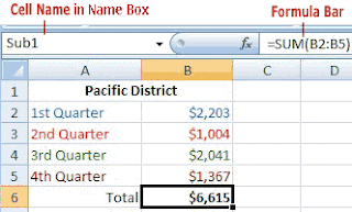
Also, when you click in a cell, if there is a cell name associated with that cell, it will display in the name box as shown in the worksheet image below.

In the example above we named the cell "Sub1" because we reference this Subtotal in a Summary worksheet.

However, after naming a cell, it seems like Excel won't let you delete or change the name! Right? Because if you click in the Name Box and type over the name or delete the name, NOTHING HAPPENS! And Excel Help doesn't seem to help.

So, how do I change or delete a cell name in an Excel spreadsheet? It's pretty easy ... it's just hidden!

So open your Excel spreadsheet and follow the directions below.

To Change a Cell Name

1. Click the Formulas tab at the top of the worksheet. Then click Name Manager on the "Defined Names" section of the ribbon. The Name Manager window displays and lists ALL of the cell names that have ever been defined in the worksheets in that workbook.

2. Click on the cell name that you want to change, and click the Edit button. The Edit Name window displays.

3. Retype the name and click OK. When finished, click Close on the Name Manager window.

To Delete a Cell Name

1. Click the Formulas tab at the top of the worksheet. Then click Name Manager on the "Defined Names" section of the ribbon. The Name Manager window displays and lists ALL of the cell names that have ever been defined in the worksheets in that workbook.

2. Click on the cell name that you want to delete, and click Delete button.

3. Click OK on the "are you sure" popup and then click Close on the Name Manager window.


Whew! By the way, our main tutorial website has just had an exciting makeover! Besides our popular beginner's tutorials such as Excel Math Basics: A Beginner's Guide and Beginner's Guide to Creating Charts in Excel, we've added tutorials on several more Excel functions, such as Nested IFs and Advanced Use of the COUNTIF Function.

Cheers!

How to Insert Multiple Blank Columns in an Excel 2007 Worksheet

The usual way to quickly insert a blank column in Microsoft Excel is to click on the column to the right of where you want the blank columns inserted, right-click, and click Insert.

You do not click in a cell, but you select or highlight the whole column by clicking on the column letter or identifier.

By default, Excel inserts a column to the left of the worksheet column that has been selected.

This works great if you want to add one blank column. But what if you need to insert multiple blank columns? Is there a better way? Yes!
If you need to insert multiple blank columns in your Excel worksheets, you MUST learn this neat method!

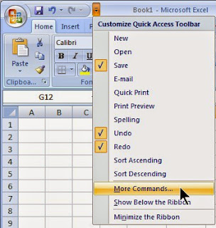
1. In your Excel document, click the little arrow after the Quick Access Toolbar in the upper right corner.
2. Click More Commands down near the bottom of the dropdown list.
3. Click Insert Sheet Columns from the list and click Add. Then click OK.
4. You just added a new icon to the Quick Access toolbar as shown in the image below.

5. NOW ... to insert multiple blank columns, highlight the column to the right of where you want the blank columns inserted and click the Insert Sheet Columns icon you just added to the toolbar. AND JUST KEEP CLICKING the icon in the Toolbar until you've inserted the number of blank columns you require!

Cool, huh.

►  Take a look at some of our other interesting posts, such as How to Display Formulas in an Excel Spreadsheet

How to Insert Multiple Blank Rows in an Excel 2007 Worksheet

A fast way to insert a blank row in a Microsoft Excel worksheet is to click on the row number that is below where you want the blank row inserted, right-click, and click Insert.

Don't click in a cell, but on the row numberat the very left of the worksheet. The entire row will highlight.

By default, Excel always inserts a blank row above the row that has been selected when following this procedure.

This works quickly if you want to add one blank line or row to a spreadsheet. But if you want to insert many blank rows, this wastes time ... and can give you a wrist cramp!

If you want to know how to quickly insert multiple rows, we provide two methods below. The first method takes a bit of set-up time, but is a faster to use if you need to insert multiple rows often. The second method is not quite as quick to use, but requires no setup.

Method One for Inserting Multiple Rows

1. In your Excel document, click the little arrow after the Quick Access Toolbar in the upper right corner. See image above.
2. Click More Commands down near the bottom of the dropdown list as shown in the image.
3. Click Insert Sheet Rows from the list and click Add. Then click OK.

There is now a new icon added to the Quick Access toolbar in the upper left corner of the Excel window as shown below.

To insert multiple rows any time in the future, click on the on the row number that is below where you want the blank row inserted and click the Insert Sheet Rows icon as many times as needed. Pretty neat, huh.

Method Two for Inserting Multiple Rows

1. In your Excel document, insert a row the usual way by clicking on the row number below where you want the blank row inserted, right-click, and click Insert.
2. Then immediately press the F4 key as many time as you need extra rows inserted.

►  Take a look at some of our related Excel posts, such as How to Display All Formulas in an Excel Worksheet

How to Display Formulas in an Excel Spreadsheet

At some point, as a Microsoft Excel user, you will need to learn how to create formulas. These may be mathematical formulas, or formulas that contain built-in functions that find averages, products, and so on.

However, when viewing the worksheet, one does not see the formula but the result of the formula.

If you click inside a cell with a formula, the formula will display in the formula bar at the top of the window. That's great if you just want to look at one single formula or function! But what if your worksheet has many formulas that you need to inspect?

We'll show you how to view all formulas on the Excel worksheet. We'll even explain how to print the spreadsheet formulas!

There are three ways to show formulas in an Excel worksheet. The three method are shown below in order of difficulty.

Display Excel Formulas - Method #1: Keyboard Shortcut

My favorite - a keyboard shortcut! If you don't have the grave or tilde symbol on your keyboard, skip to Method #2.

Open the spreadsheet. Then hold the Ctrl key while pressing the grave (`) or tilde (˜) key. On many Windows keyboards the grave is the "capital" of the number 6, and the tilde is the "capital" of the number 1.

Pressing these two keys will toggle back in forth between displaying the formula values and the formulas themselves.

Display Excel Formulas - Method #2: the Excel Ribbon

If you don't like keyboard shortcuts, this method works quickly in Excel 2007, 2010, and newer versions:

Click the Formulas tab on the Excel 2007 ribbon.
In the "Formula Auditing" section to the right, click Show Formulas.

To hide the formulas and return to the worksheet, follow the same instructions above and click Show Formulas to un-select it.

Display Excel Formulas - Method #3: Excel Options

This method is the most cumbersome. But it is another way to show formulas.
Click the Office button in the upper left corner and then click the Excel Options button in the lower right.

Click Advanced on the left sidebar and scroll down to Display options for this worksheet.

Click to select Show formulas in cells instead of their calculated results and click OK.

Don't forget to remove the check mark in this box when you want Excel to display the calculated results once again instead of the formulas.
Note: When the formulas are displaying on the worksheet instead of the normal worksheet values, the "show formulas" box will be checked in the Excel Options window, and the "show formulas" will be selected on the ribbon.

For many Excel tutorials, check out our main website: Microsoft Office Version and Windows Version Compatibility Chart is our newest tutorial. Another popular tutorial for newer (or rusty!) Excel users is Excel Math Basics: A Beginner's Guide.

We hope this helps. Cheers!

►  Take a look at some of our other interesting posts, such as Quickly Enter Time & Date in Excel.

A Dozen Sample Math Formulas for Microsoft Excel

In Microsoft Excel, the math formula is entered in the cell where you want the results displayed. The symbols for adding, subtracting, multiplying, and dividing are: + - * /

You do not have to use capital letters when keying in cell references - Excel will capitalize them for you. But you do need to understand Mathematical Order of Operations..

This article provides examples of the Order of Operations for your practice. If you're unsure, first read our article Mathematical Order of Operations. (Parentheses, Exponents, Multiplication/Division, and Addition/Subtraction).

You might find that you can remember the mathematical Order of Operations by remembering: Please Excuse My Dear Aunt Sally . . . or Sue, or Sylvia ...

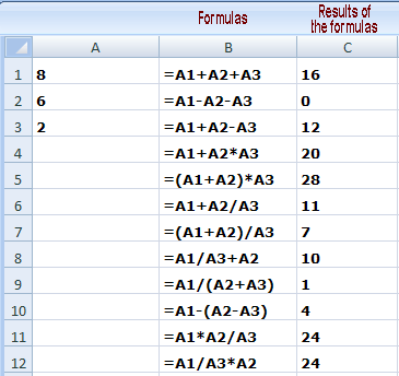
Our 12 formulas have been entered into the Excel worksheet shown below. The cell values we are referencing in the formulas are in Column A, the formulas are displayed in Column B, and the values the formulas produce are shown in column C.


Example #1 (B1): =A1+A2+A3: calculate from left to right: 8 + 6 + 2 = 16
Example #2 (B2): =A1-A2-A3: calculate from left to right: 8 - 6 - 2 = 0
Example #3 (B3): =A1+A2-A3: 8 + 6 - 2 = 12
Example #4 (B4): =A1+A2*A3: the multiplication, A2 x A3, is done first, so 8 + 12 = 20
Example #5 (B5): =(A1+A2)*A3: math inside parentheses is always done first, so 14 x 2 = 28
Example #6 (B6): =A1+A2/A3: the division, A2 ÷ A3, is done first, so 8 + 3 = 11
Example #7 (B7): =(A1+A2)/A3: inside the parentheses is calculated first, so 14 ÷ 2 = 7
Example #8 (B8): =A1/A3+A2: since division is done before add/subtract, proceed from left to right: 4 + 6 = 10
Example #9 (B9): =A1/(A2+A3): inside the parentheses is calculated first, so 8 ÷ 8 = 1
Example #10 (B10): =A1-(A2-A3): parentheses first, so 8 - 4 = 4 (compare with Example #2)
Example #11 (B11): =A1*A2/A3: since multiply and divide are equal in "weight," just proceed from left to right: 8 x 6 is 48; then 48 ÷ 2 = 24
Example #12 (B12): =A1/A3*A2: calculating from left to right: 8 ÷ 2 = 4; then 4 x 6 = 24

►  Take a look at some of our other interesting posts, such as Cleaning Up Disk Space

Mathematical Order of Operations and Excel

This blog post covers the Mathematical Order of Operations that Microsoft Excel will use to interpret formulas and functions.

In order to enter formulas into Excel worksheets, you have to know how Excel will interpret the formulas you enter. If you are new to Excel math, we highly recommend reading Excel Math Basics on our main website.

There is a TRICK to remember the Order of Operations! Just remember this easy phrase:

Please Excuse My Dear Aunt Sally

If you have an Aunt Suzette (great name) or an Aunt Sarsaparilla (not so great...), then remember that phrase! So, how does this help us understand order of operations for Excel?

The first letter of the words, highlighted in red, represent Parentheses, Exponents, Multiplication, Division, Addition, and Subtraction. And this is the order in which the operations are carried out. All operations are performed from left to right.

So, given any formula, the following describes how the order of operations are performed:

1. First, go through the formula from left to right and calculate any math inside of parentheses
2. Go through the formula a second time and calculate any Exponents. The exponent symbol is a caret ^
3. Go through the formula a third time and calculate Multiplication and/or Division. Multiplication is indicated by * and division by /
4. Go through the formula one last time and calculate all Addition and/or Subtraction.

Note: Even though the Aunt Sally phrase may imply that Multiplication is done before Division, that is not true. They are performed during the same step, from left to right. The same is true regarding Addition and Subtraction.

Let's practice with a rather complication formula to illustrate each operation: (2*4)+3^2-8/4

1. Pass 1 - Parentheses: Inside some parentheses we have 2*4, which equals 8. Now our expression reads: 8+3^2-8/4
2. Pass 2 - Exponents: In our formula we have 3^2, or 3*3 which equals 9. Now our expression reads: 8+9-8/4
3. Pass 3 - Multiplication and/or Division: 8/4 equals 2, so now our formula reads: 8+9-2
4. Pass 4 - Addition and/or Subtraction: proceed from left to right and our answer equals 15

You can type =2*4+3^2-8/4 into a cell in an Excel worksheet and Excel will use the Order of Operations properly and display, in the cell, the value of 15.

You can, however, use parentheses to help you from getting confused; i.e. =(2*4)+(3^2)-(8/4).

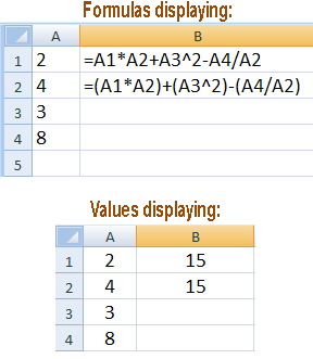
Lastly, since cell references are typically used in formulas instead of just numbers, let's look at our sample formula in an Excel spreadsheet where the numbers, except the exponent, are stored in cells: A1=2, A2=4, A3=3, and A4=8.



As shown in the top part of the image below, we typed the formula two ways: without any parentheses (in cell B1) and with some parentheses (in cell B2). In the lower part of the image, you can see that Excel calculates a value of 15 in both instances.

Cheers!

Hot Tip to Quickly Enter Date and Time in Microsoft Excel

It is often very useful when creating an Excel worksheet to post the data somewhere on the worksheet. This is especially true if you have multiple versions of the same worksheet.

However, it takes time to format a cell and then type in the date.

Today we share with you a great keyboard shortcut that will allow you to enter the current day's date, or time, or BOTH in a spreadsheet as quick as can be.

Do remember that Excel always uses the current date and time from your computer, so make sure they are accurate.

How to Enter the Date in an Excel worksheet with a Keyboard Shortcut

Click on the cell in which you want the date to appear. Then press Ctrl + ;   (In other words, press and hold the Ctrl key while you press the colin or semicolon key). Presto!

How to Enter the Time in an Excel worksheet with a Keyboard Shortcut

To quickly get the time in a spreadsheet, click on the cell and press Ctrl + Shift + :   (Press and hold the Ctrl and Shift keys and then press the colon or semicolon key).

How to Enter the Date AND Time in the Same Worksheet Cell with Keyboard Shortcut

You can enter BOTH the date and time in one cell if you type the keyboard shortcut for the date first, press the space bar, and then type the keyboard shortcut for the time. This is real cool if you create a lot of spreadsheets!

For a list of the most popular keyboard shortcuts for Excel, please see our tutorial Microsoft Excel: Cool Keyboard Shortcuts.  Our main website has many other tutorials for Excel beginners, such as Excel Made Easy: A Beginner's Guide and more advanced tutorials, such as the ones that explain how to use Excel's most popular built-in functions. Don't miss our newest tutorial, Microsoft Office Version and Windows Version Compatibility Chart..

Cheers!

►  Take a look at some of our other interesting posts, such as How to Display Formulas in an Excel Worksheet

Using the Paintbrush (Format Painter) in Microsoft Office

A lot of people have never noticed the little paintbrush icon that can be seen on a toolbar in both Microsoft Word and Microsoft Excel. It's the little icon shown in the image at right. 

Microsoft calls it the Format Painter and it is a fabulous, handy tool for quickly duplicating styles and formatting of text.

In Office 2007 and later versions, the Format Painter resides on the Clipboard section (far left) of the Home tab of the ribbon. In Office 2000 or below, it is located on one of the standard toolbars.

The Format Painter allows you to copy the font style, size, and color from one part of the document and apply it to one or more other words, paragraphs, and more. It is a great productivity tool!

Let's learn how to use the Format Painter for duplicating one instance or multiple instances.

Using the Format Painter to Make One Duplicate

1. Highlight a portion of the paragraph that has already been formatted
2. Click the Paintbrush icon once
3. Carefully highlight the new text you want styled like the original, and then release the mouse key

Presto! It is formatted exactly like the first paragraph.

Using the Format Painter for Multiple Duplication

1. Highlight a portion of the paragraph that has already been formatted and whose formatting you want to duplicate elsewhere in the document.
2. Double-click the Paintbrush icon.
3. Proceed to an area of text you wish to format like the original. Very carefully highlight that text. Then release the mouse button and the text will be formatted. Notice that the Format Painter icon stays activated.
4. Proceed to the next paragraph, word, or section of text you wish to format and repeat. Keep carefully highlighting and formatting text until finished.
5. When completely finished, click the Format Painter icon once to deactivate it. It should no longer be highlighted.

Why do we emphasize "very carefully"? You may have noticed that sometimes Microsoft Word can be touchy when highlighting and jump around a bit. If you accidently highlight the wrong text, immediately Undo the action. You can undo the action by clicking the left-facing circular arrow up on the top toolbar, or use the keyboard shortcut Ctrl + Z - meaning hold the Ctrl key while pressing the "z" key.

Learn how to use the Format Painter and let it increase your productivity!

How to Change Cell or Column Widths in Excel

There are a variety of different ways that you can change the width of cells or columns in Microsoft Excel. Knowing these different options will give you greater control over the structure of your Excel worksheet.

To change a single column width visually:
Place the cursor over the right vertical column separator. For example, to make column D wider, place the cursor on the column separator between columns D and E.

Then, when the cursor changes to a plus sign, click your mouse and drag left or right.

To determine the width value of a column:

If you want to know the width of a column, place the cursor on the right vertical separator line of the column. When the cursor changes to a + sign, press and hold the left mouse button. Excel will show you the column width value.

To change a single column width using a value:

Place the cursor over the column heading (A, B, etc.). When the cursor changes to a downward arrow, right click and click Column Width. Enter a number, and click OK.

In general, for the default fonts of Cambria (Excel 2007) and Arial (prior releases), with a font-size of 10 and a column width of 10, the column will hold about 10 numbers.

To have Excel automatically size a column width:

To ask Excel to automatically define the width of a column to fit the widest value, double-click on the vertical separator bar on the right side of the column heading.
Optionally, in Excel 2007, click on the column heading, click Format on the Cell section on the Home tab, and click AutoFit Column Width.

To make every cell in the spreadsheet the same width:

First, select every cell in the worksheet by clicking the “Select All” square - which is the upper-most portion of the spreadsheet located above row 1 and to the left of column A. Then find the Cells section of the Home tab. Click Format, click Column Width, and enter a number.

To have Excel automatically size all the column widths:

To ask Excel to automatically define the width of each column to fit the widest value, first, select every cell in the worksheet by clicking the “Select All” square - which is the upper-most portion of the spreadsheet located above row 1 and to the left of column A. Then, on the Cells section of the Home tab, click Format and click AutoFit Column Width.

If you are new to Excel, check out our popular tutorial Excel Made Easy: A Beginner's Guide at KeynoteSupport.com. We also have great tutorials for advanced Excel users.